Hello GeoLens
Script: 0_hello_geolens.py
The fastest end-to-end tour of the geometric-lens workflow: load a lens, run the classical optical analyses, and render an image through it with both ray tracing and PSF-map convolution.
What it demonstrates
- Loading a
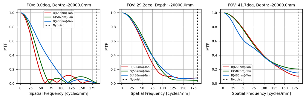
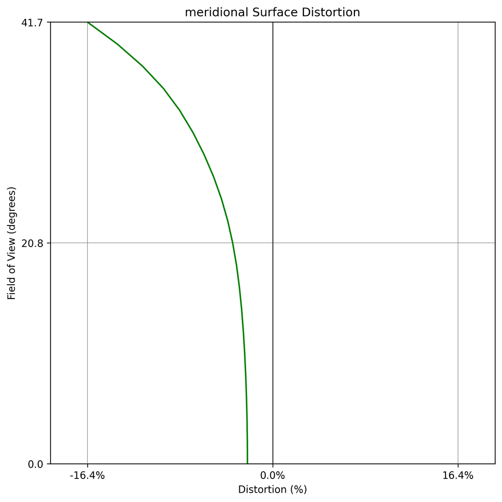
GeoLensfrom JSON (Zemax.zmxand Code V are also supported). - The classical evaluation plots: layout, spot diagram, MTF, distortion, and relative illumination (vignetting).
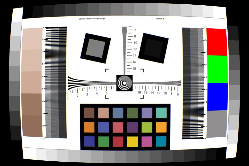
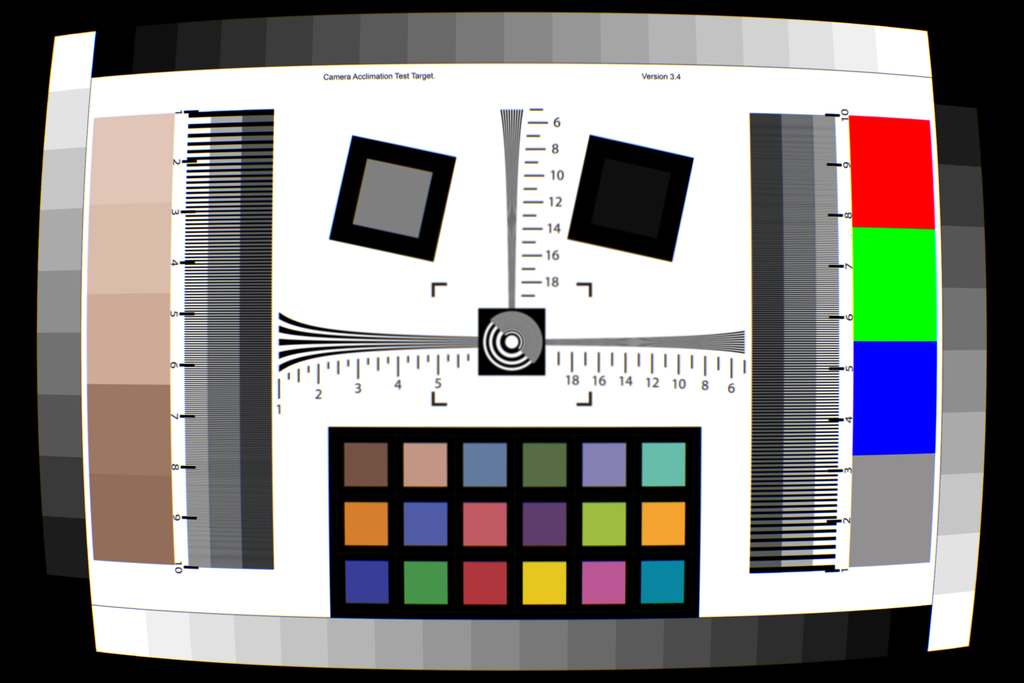
- Two rendering paths: per-ray
ray_tracingand spatially-varyingpsf_map.
Run
Key code
from deeplens import GeoLens

lens = GeoLens(filename="./datasets/lenses/cellphone/cellphone80deg.json")

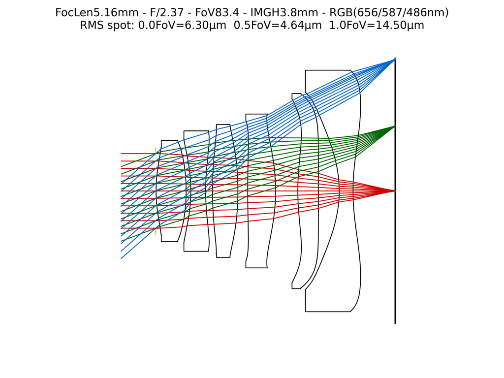
lens.draw_layout(filename="./lens.png")
lens.analysis_spot()
lens.draw_spot_radial(save_name="./lens_spot.png")
lens.draw_mtf(depth_list=[lens.obj_depth], save_name="./lens_mtf.png")
lens.draw_distortion_radial(save_name="./lens_distortion.png")
lens.draw_vignetting(filename="./lens_vignetting.png", depth=lens.obj_depth)

# Image simulation at the sensor resolution
lens.set_sensor_res((3000, 2000))
img_ray = lens.render(img, depth=DEPTH, method="ray_tracing", spp=8)
img_psf = lens.render(img, depth=DEPTH, method="psf_map", psf_grid=(30, 20))
Results
Lens layout
Optical analysis
| Spot diagram | MTF |
|---|---|
 |
 |
| Distortion | Vignetting |
|---|---|
 |
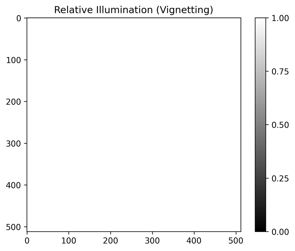 |
Image simulation
| Ray tracing | PSF map |
|---|---|
 |
 |